Basic Computer Vision Tasks

2023-11-28 3217 words 16 minutes

/posts/projects/basic-computer-vision/images/hough4.png

Contents

The following are a few of the most interesting projects completed for the Intro to Computer Vision course which implement several basic computer vision tasks. The results seen in each of these reports were produced by implementing the relevant algorithms from scratch using NumPy. OpenCV was only used for loading images or drawing on top of images.

Canny Edge Detection

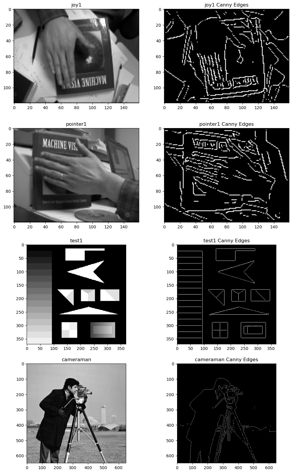
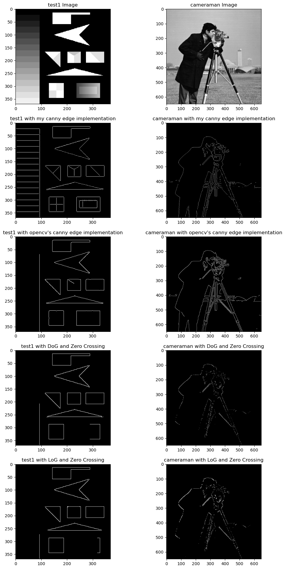
The purpose of this project was to implement the Canny Edge detection algorithm which consists of 5 main steps: gaussian smoothing, calculating the image gradient, selecting thresholds for the gradient magnitude, thinning the gradient magnitudes by suppressing non-maxima, and finally, linking strong edges along weaker edges.

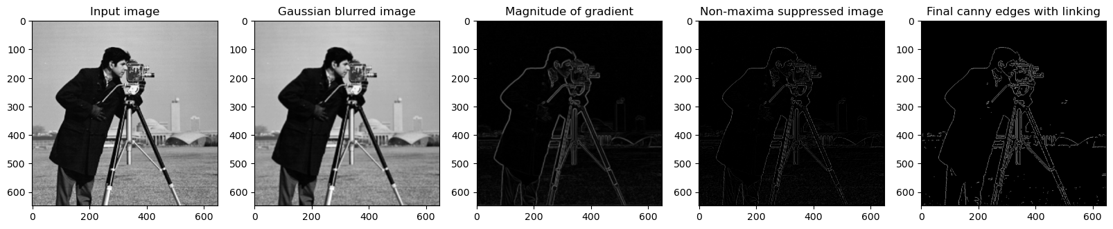
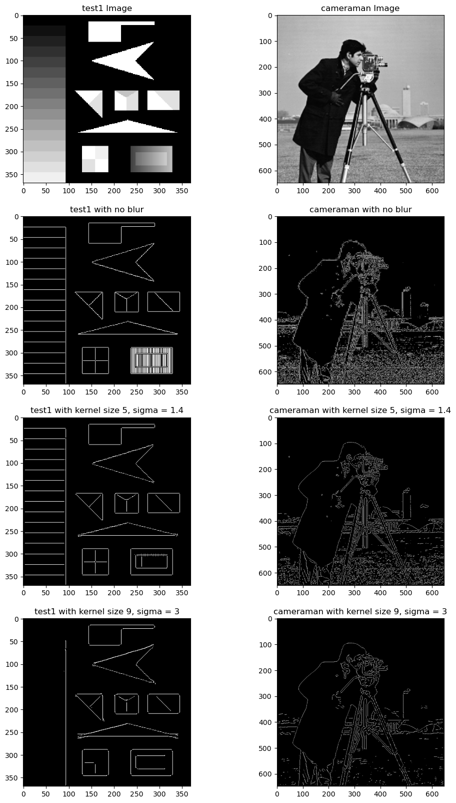
/posts/projects/basic-computer-vision/images/mp5_cameraman_steps.png — Figure 1: A preview of the results of applying each step of the canny edge detection algorithm.

The first step is simple: we first generate a gaussian kernel by defining a square numpy array of a given size. Then, we fill the array by sampling the gaussian function with a given standard deviation sigma at each pixel where the input is the pixel’s distance from the center of the array. Next, we convolve the gaussian kernel with the image, treating points that are beyond the edge of the image as 0. However, in my implementation, we actually cross correlate the kernel. Since the kernel is symmetric, the result will be identical.

/posts/projects/basic-computer-vision/images/mp5_blurring.png — Figure 2: Applying two different gaussian kernels to test images. Note how the size of the kernel and the value of sigma directly affect the blurriness of the output. Also note that this is an expensive operation: O(imageHeight*imageWidth*kernelHeight*kernelWidth), so a larger gaussian kernel is quadratically more expensive to apply.

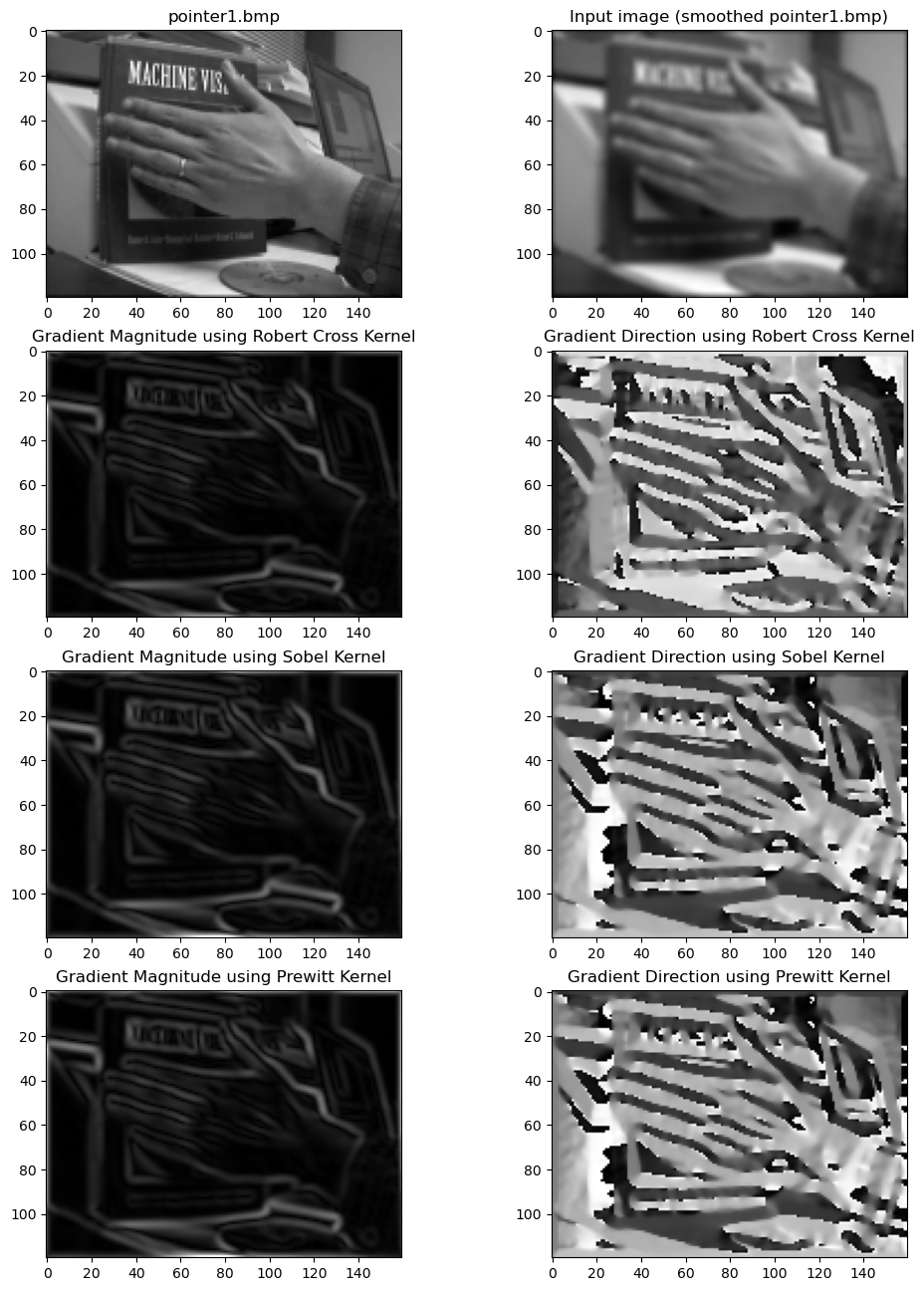
The next step is to calculate the image gradient. To do so, we convolve the image with a gradient kernel like robert cross, sobel, or prewitt. We have to compute the gradient along X and Y so we actually have to convolve with the X and Y variants of each of the kernels. Then, we can determine the magnitude of the gradient at each pixel (the square root of the sum of the squared x and y components) and the direction of the gradient at each pixel (by calculating the arctangent of y/x). Note that for this implementation, again, I used cross correlation instead of convolution. This should again give the same results for magnitude and flipped results for the x direction gradient which will not matter since, in a later step where the directions are used, we check both sides of the gradient regardless.

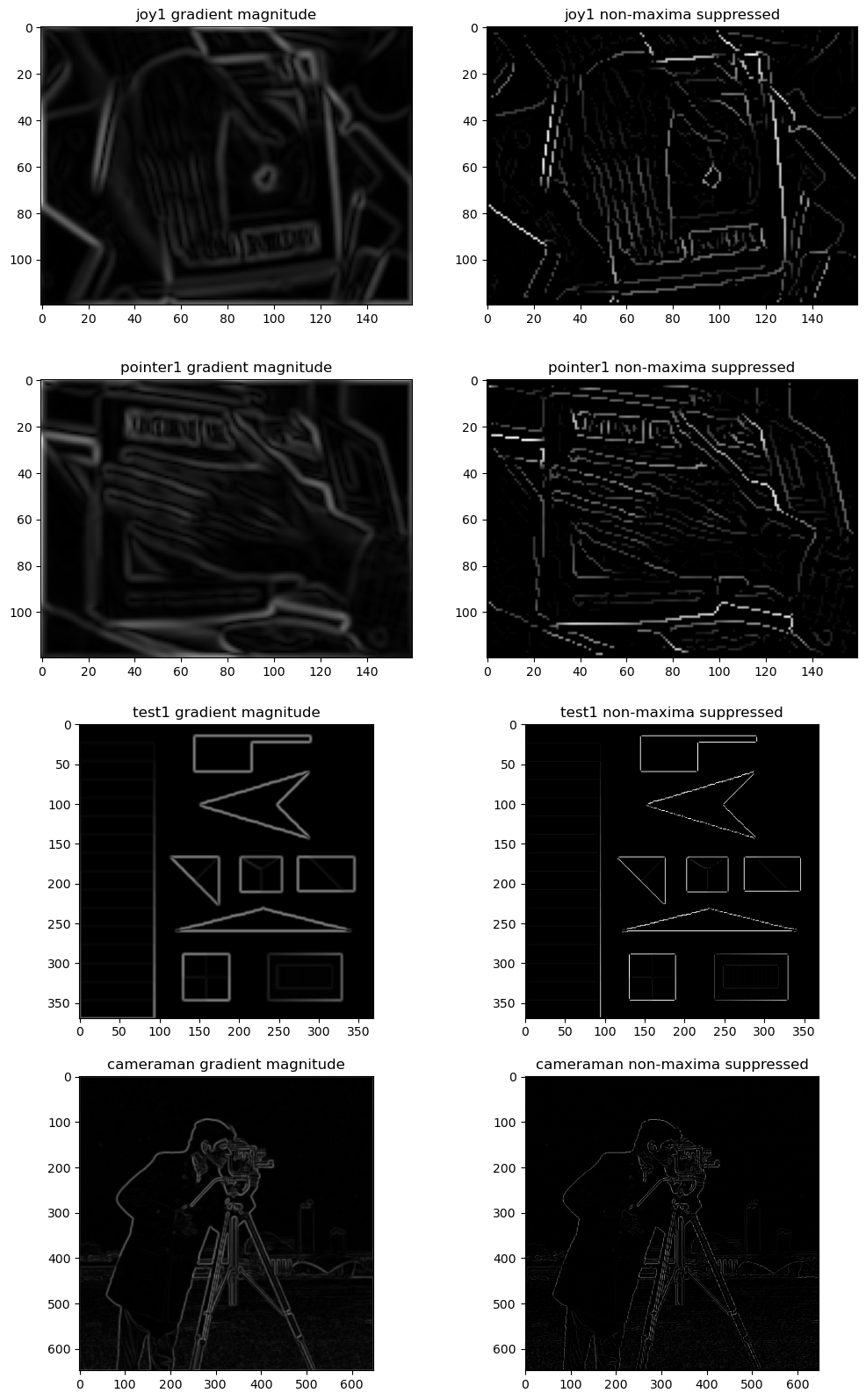
/posts/projects/basic-computer-vision/images/mp5_gradients.png — Figure 3: The results of running the image gradient function using different gradient kernels. They all produce comparable results so I went with Robert Cross since it is the smallest kernel to apply (2x2).

After we have the image gradients, we can thin the gradients by suppressing non-maxima. The basic idea is simple. At each pixel of the magnitude of the gradient, if it is not the local maximum, set it to 0. In practice, this was implemented using a lookup table and the gradient direction information. Effectively, at each pixel, we use the angle of the gradient to determine which pair of surrounding pixels we should compare the current pixel to. Note that since we are looking down each side of the gradient, we can compress the lookup table to only include half the directions and add pi to each negative entry in our gradient direction array. If the current pixel is greater than both of its neighbors along the gradient direction, set its result to the original magnitude of the pixel, else set it to 0.

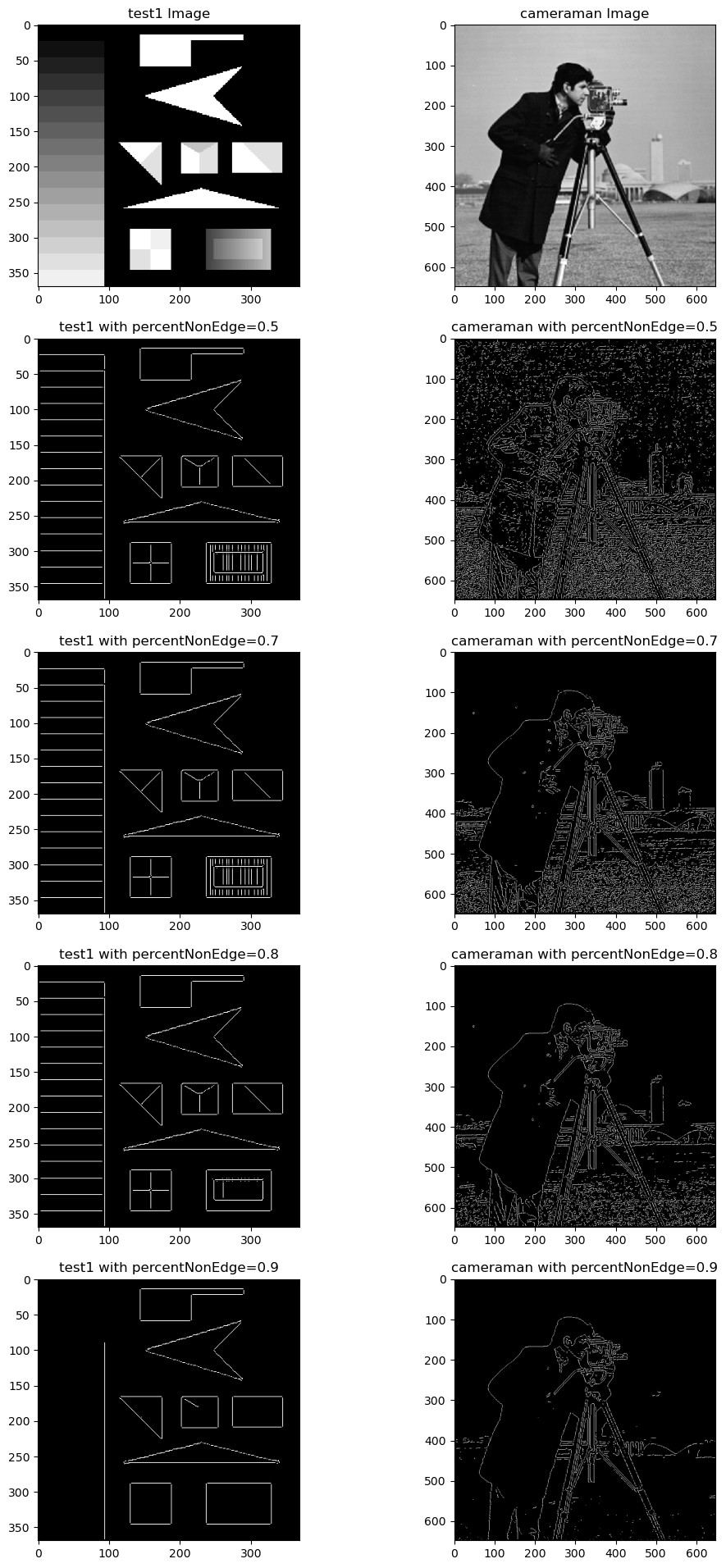
/posts/projects/basic-computer-vision/images/non-maxima-suppressed.png — Figure 4: The effect of applying non-maxima suppression to the images. We can see that this process already gives pretty good results with thin edges. However, the canny edge detector includes one last step to threshold the edges and create a set of well-defined edges.

The last step is a combination of determining the threshold for the edges then linking those edges. To determine the threshold in pixel intensity, we create a histogram of the gradient magnitude image then use an arbitrary threshold that represents the percentage of pixels that are non-edges to determine at which pixel value the threshold for pixel edges should be. Note the use of the original gradient magnitude and not the non-maxima suppressed gradient magnitude to determine the threshold! We define strong edges as all intensities above the threshold and weak edges as all other intensities above half the threshold. Once we have the threshold, we can perform edge linking on the non-maxima suppressed image. To perform edge linking, we begin by iterating through every pixel. Within each pixel, we run a recursive edge linking function. In the recursive function, if the current pixel is a strong edge, we set it as 255 in the result then check all 8 of its neighbors and call the recursive function on them. If it is a weak edge but the recursive call came from a strong edge, then we set it as 255 in the result and recursive call the function on all of its neighbors. In this manner, we extend strong edges along the weak edges that connect to them.

/posts/projects/basic-computer-vision/images/cannys.png — Figure 6: Results of applying my implementation of the canny edge detection algorithm to each of the provided test images. Each of these images used slightly different parameters which I had to determine experimentally.

/posts/projects/basic-computer-vision/images/dif_blurs.png — Figure 7: Testing with different blur kernels. Here we can see that without any blurring, we get really noisy results. As our blur kernels get larger, we lose a lot of finer details in our edges (i.e., our edges look rounder).

/posts/projects/basic-computer-vision/images/dif_non_edge.png — Figure 8: Testing with different percentNonEdge. Here we can see that the resulting edges still maintain the same level of detail in terms of their shape but adjusting the value changes the threshold to noisy edges.

/posts/projects/basic-computer-vision/images/dif_edge_methods.png — Figure 9: Comparison to other edge detection methods including OpenCV’s implementation of Canny Edge Detection and zero crossing with Difference of Gaussians and Laplacian of Gaussians. Both zero crossing methods produce similar edges but the results tend to be more noisy and seem to miss more edges (at least with the parameters used). The OpenCV implementation produces similar results to my implementation but seems to have a modified edge linking step resulting in edges that look thicker and smoother.

Hough Transform Line Detection

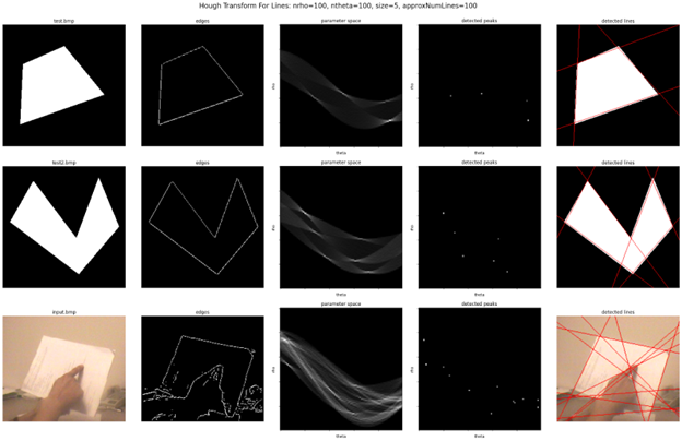
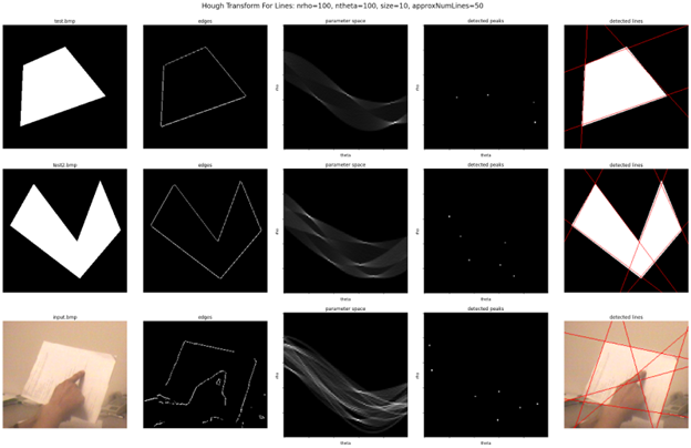
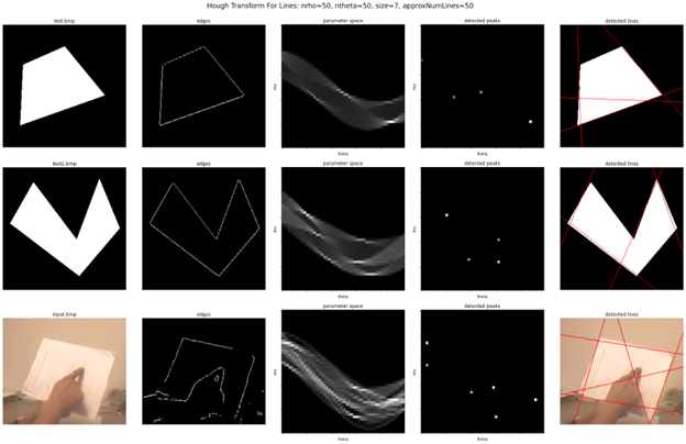
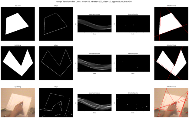
The purpose of this project was to use a Hough Transform to detect lines from the edge map of an image. The general idea of the Hough Transform is to first input the edges of an image (e.g., edges detected using canny edge detection), then convert all points in the edge map to curves in rho-theta parameter space, then determine the significant intersections in that parameter space, and finally map those points in parameter space back to lines on the original image.

In my implementation, I first detect edges using the canny edge detection algorithm I made for MP#5. Therefore, the first major task for this MP was to create the parameter space. To do so, I first created an array of zeros of size nrho times ntheta where nrho was the quantization for the distance parameter rho, and ntheta was the quantization for the angle parameter theta. Now, I had to determine the range of values that would be mapped to each bin in the parameter space. For my implementation, the rho parameter ranges from -maxDist to +maxDist where maxDist is the diagonal extent of the image. The theta parameter ranges from -pi/2 to pi/2. To determine the range for each bin, I simply divided the length of the range by the quantization of each parameter. Next, to fill in the parameter space, I iterated through each of the edge points in the edge map. For each edge point, I iterate through all the thetas in my parameter space and determine their corresponding rhos using the equation: rho = x*cos(theta) + y*sin(theta) where x, y are the coordinates of the edge in the original image. For each value of theta, we count a vote in the corresponding value of rho. Note that I would use the value of theta at the center of each bin in hopes of creating a more accurate mapping between theta and rho.

Once we complete this process for all edge points, we have our votes for lines in the parameter space. The next step is to determine the significant points (or peaks) in the parameter space. My particular implementation for this was composed of two steps: thresholding, and finding local maxima. To threshold, I used the same thresholding algorithm I created for MP#5 where we pass in a percentNonEdge to determine the threshold from the histogram. Except this time, percentNonEdge was determined by inputting the approxNumLines variable such that percentNonEdge = 1 - approxNumLines/size of image. The general idea of this is to pick out the most significant points in the parameter space. However, there may be many such significant points close together in the parameter space due to noise in the edge map or limits due to quantization. Therefore, we would then find the local maxima of the remaining points. To do so, we would iterate through every bin in the parameter space. If a given bin was the local maximum in a window of size size, it would be kept as a detected peak, else it would be set to 0. This is definitely not the best method for detecting significant points of the parameter space, but it seemed to work well enough for our test cases.

The last step is to convert the detected points back to lines in the image space and draw said lines over the original image so we can check our work. First, we had to extract the rho and theta value for each peak. Doing so is straightforward – we just get the bin indices for rho and theta and map them back to the corresponding values. One thing to note is that I, again, mapped them back to the center of each bin by adding a factor of ½ of the stride of each bin. Then, to draw the lines, I used OpenCV’s line drawing function cv2.line to draw a line using two points along the corresponding line for each peak in the parameter space. To determine the points, we first use x = rho*cos(theta) and y = rho*sin(theta) to get an initial point then move along an offset (equivalent to the diagonal extent of the screen plus 1 to guarantee the ends of the line are off the image) along the slope of the line in either direction.

Results

/posts/projects/basic-computer-vision/images/hough1.png — Figure 1: The results of the Hough Transform using the default parameters for my functions. From left to right, each column represents the original image, the edge map of the image, the parameter space (where the y axis is rho from -maxDist at the top to +maxDist at the bottom and the x axis is theta from -pi/2 on the left to pi/2 on the right), the detected peaks from the edge map, and finally the detected lines drawn over the original image. The title of each figure has the quantization of rho and theta that was used, the size of the window used to determine the local maxima, and the number of lines used to set the threshold for the peaks. We can see from this example that the default parameters I used worked well for the first two test cases but there were a lot of noisy lines in the final image.

/posts/projects/basic-computer-vision/images/hough2.png — Figure 2: Adjusting parameters to get better edge results. For this example, I still used the same quantization of nrho=100 and ntheta=100 as I had used in Figure 1 but increased the size of the local maxima window from 5 to 10, increased the threshold for the parameter space by lowering approxNumLines from 100 to 50, and increased the percentNonEdge from 0.8 to 0.9 for canny edge detection to remove the noise in the edge map of the last test image. From these changes, the result for the first two test cases was identical but the final test case results were much improved and far less noisy.

/posts/projects/basic-computer-vision/images/hough3.png — Figure 3: Here, I lowered the quantization from nrho=ntheta=100 to nrho=ntheta=50. Here, we can see the Hough Transform starts to break down a little bit. Some of the lines it detects still seem accurate but tend to be more skewed, especially in terms of angle compared to the true edge. We can also see that it picks up an erroneous edge in the first test case.

/posts/projects/basic-computer-vision/images/hough5.png — Figure 5: For this example, nrho=50 but ntheta=100. Now, as we expect, the edges that are detected are fairly close in terms of angle, but the lines tend to be more offset from the edges as can be seen especially in tests 1 and 2. We also see my peak detection failing in this case as there are several local maxima that are fairly close in the last test image despite the window size already being fairly large (size=10) and many edges are missing despite being visible in the parameter space for test 2.

Template-Matching Based Target Tracking

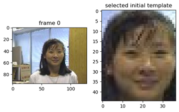
The goal of this project was to track a moving target in a video (i.e., a series of images) using a template matching approach. The basics of the algorithm are simple: we first initialize a template, say by manually picking a region from the first frame of the video (see figure 1). Then, to determine the position of the object in the next frame, we slide the template over a region around the previous position of the object and determine which position within that region best matches the template based on a given criteria. Potential criteria include: the minimum of the sum of squared differences, or the maximum of the cross correlation or normalized cross correlation. Once we have the best matching position, we draw a bounding box around that position of the same size as the template that was used. In between frames, we can optionally update the template to be the matching region from the previous frame. In my particular implementation, I take the best match of both the initial template and the updated template to determine the new best match to help avoid having the detection stray too far from the true target. By repeating these steps for all frames, we should be able to track the movement of the target within the frame.

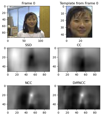
/posts/projects/basic-computer-vision/images/mp7-1.png — Figure 1: Picking an initial template from the first frame.

When we slide the template over a region of the image, we get an intermediate representation of all the positions that the template could have been in and the corresponding value of the criterion used. In figure 2, we can see the intermediate representation for the first frame using all of the different criteria used in this MP. Note that for sum of squared distances (SSD), we want the minimum since we want to minimize the difference. However, for normalized cross correlation (NCC), we want the maximum since similar pixels should result in higher correlation. One caveat is that for cross correlation (CC), we can end up with large values despite not having a good match because the pixel values themselves are large. This is why we use NCC instead and is why we should expect CC to perform poorly. Note that for my implementation, I implemented NCC and DiffNCC where the only difference between the two is that NCC uses the actual pixel values while DiffNCC uses the offset of the pixel values from the mean of the image and the template.

/posts/projects/basic-computer-vision/images/mp7_2.png — Figure 2: Intermediate representations of applying different criteria to the images. Note that for these examples, we are sliding the template over the entire image so the size of the intermediate representations are the image dimensions minus the template dimensions.

For my implementation, there are two additional parameters that affect the compute time and results. The first is updateTemplate, which if true, will update the template to be the last matching region of the image and will use both the initial template and the updated template to determine the next best match. This doubles compute time since we have to compare both templates but it does to a small extent, help steer the detection back to the true target in case the matches start to deviate too far. This is helpful because one downside of having the template update is that it tends to propagate errors. In many test cases where updateTemplate was set to True, I noticed the detection would veer off the target and end up focusing on the wall in the background or the blinds or stick to detecting, say, half of the target’s face. In these scenarios, comparing against the initial template increases the likelihood of moving back to the true target.

The other adjustable parameter is the searchSize. This ultimately determines the size of the intermediate representation and the distance to search from the previous position of the target in the image. If it is set to zero, then all possible positions will be searched. Having a large searchSize increases the compute time (since compute will be proportional to searchSize squared) and increases the distance the object is “allowed” to move between frames (i.e., the maximum distance the object can move and still be accurately detected). However, having it too large increases the chance of false detections and can make the tracking more jittery as it bounces around between best matches. I found setting it to 5 gave the best results and was fast to compute.

Under otherwise equivalent settings (updateTemplate=False, searchSize=5), CC was fastest at just 0.25 seconds to process all 500 images, followed by SSD which took 0.36 seconds, then NCC which took 0.64 seconds and finally, DiffNCC was by far the slowest at 3.44 seconds. This matches what we should expect for the rankings of speed. CC is the fastest because we only do a single round of element-wise multiplication. SSD is second because we have to do element wise subtraction then multiplication. NCC is slower because we have even more operations but importantly, can ignore needing to take a square root if we leave the numerator and denominator squared. DiffNCC is the slowest primarily because of the square root in the denominator which we need to take because the numerator can be positive or negative.

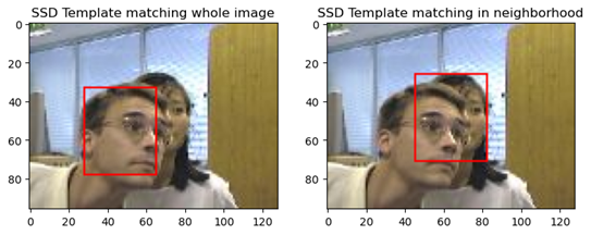
Results and Occlusion

Regarding the results, by far the best results I got were using SSD without updating the template between frames and setting the search size to 5. That is the result shown in the video below. We can see in figure 3 that it was the combination of using SSD and checking only in the neighborhood which allowed the tracking to stay fixed to our target despite occlusion. All other criteria failed with otherwise equivalent settings as did using SSD on the whole image for just that frame.