This project was part of an independent study where I, along with a few other students, were extending a pre-existing ray tracer made by a PhD student, Kelly Jiang. What follows is the report I submitted for the project that runs through the different camera systems I implemented with a brief explainer and example results of each.
Introduction
Ray tracing has the unique advantage of easily simulating many different types of cameras. All we need is to provide the appropriate outgoing ray from the camera system and let the ray tracer take care of the rest. The ability to simulate different types of cameras opens up many artistic possibilities when making rendered images or animations. For instance, one of my favorite artistic uses of a realistic camera system can be seen in Toy Story 4. In this movie they modeled several different types of cameras including the simpler spherical lens camera (which are discussed later in this report) as well as more complex split-diopter (fig. 1) and anamorphic lenses. The YouTube channel Nerdwriter has a good explainer on the artistic impact of these lenses in this video. Ofcourse, realistic camera simulations can also be useful for research. For example, the Dahl lab at Northwestern is currently in the process of simulating images from their bubble chamber. The cameras peer into the bubble chamber through a series of relay lenses which need to be accurately simulated for correct results.
 Figure 1: A frame from the movie Toy Story 4 featuring the split diopter lens.
This report will cover 4 different camera types that were implemented following chapter 6 of the book Physically Based Rendering: From Theory to Implementation (PBRT), available online here. For more information on any of these camera models, please read the corresponding section of the book. Note that unless otherwise stated, all images of the 3-sphere scene were taken from the same position and looking in the same direction with a sample rate of 256 samples per pixel and the gamma set to 2. In addition, a border has been added to distinguish the edges of the images since the background is also white. Finally, full resolution images can be viewed from this google drive.
Pinhole Camera
This implementation of the pinhole camera model assumes that the film plane is in front of the pinhole. Then, the rays originate from the location of the camera and the direction is determined by sending the ray in the direction of a given pixel on the film plane. Spatial anti-aliasing is done by randomly choosing a position within the pixel to sample. The user can set the field of view and the aspect ratio (though it is usually automatically determined by the resolution), as well as the distance to the near-clipping plane. The field of view and aspect ratio determine the size of the pixel grid at which the rays are shot and hence the range of angles covered by the camera.
In reality, we would expect pinhole cameras to produce really dim images or require long exposure times since only a few light rays will make it past the pinhole to produce the image. However, for this ray tracer we are explicitly only shooting rays that are simulated as passing through the pinhole. In addition, we do not have any exposure time settings for this camera (at least not for this branch of the project) so we would not be able to simulate that result regardless.
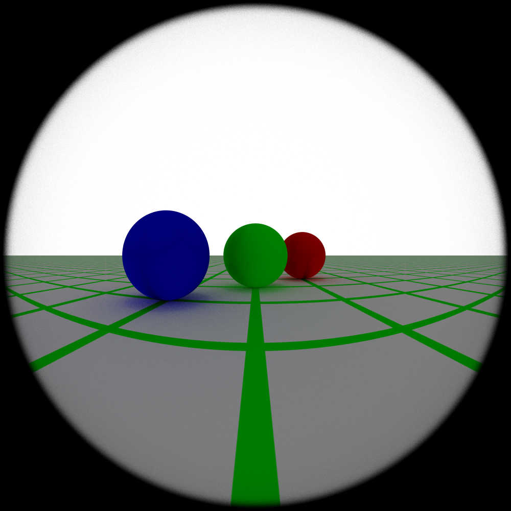
A defining characteristic of pinhole cameras is that, since they have an infinitesimal aperture, everything is in focus. We can see that explicitly in fig. 2.
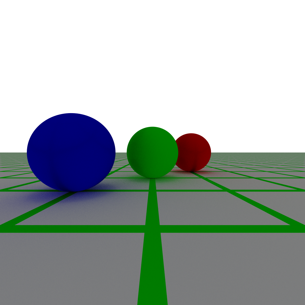 Figure 2: A pinhole camera image with a 90 degree field of view. Notice that all three spheres are in focus. We can also see the effect of antialiasing as we look at the grid approaching the horizon.
Environment Camera
The environment camera operates on a similar principle to the pinhole camera except that, instead of getting the ray direction by drawing a vector from the camera origin to a point on the film plane, we now determine the ray direction via a point on a sphere that encapsulates the camera. The environment camera effectively maps the full 360 degree field of view from a point on the scene to a rectangular image. This also means that the environment camera captures all the incident light on a point in the scene.
While it is not explicitly required, the aspect ratio for the resolution of the environment camera should be 2:1. This is because the environment camera is mapping 0 to 2Pi radians of azimuthal angle along the x axis of the camera and 0 to Pi radians of the inclination angle.
Images produced using the environment camera can be viewed by projecting the image back onto a sphere and rotating a fixed camera. Doing so allows you to effectively “look around” at what a scene looks like from a given position. While this is not explicitly built into this rendering, an online tool can be used to view the image such as this one.
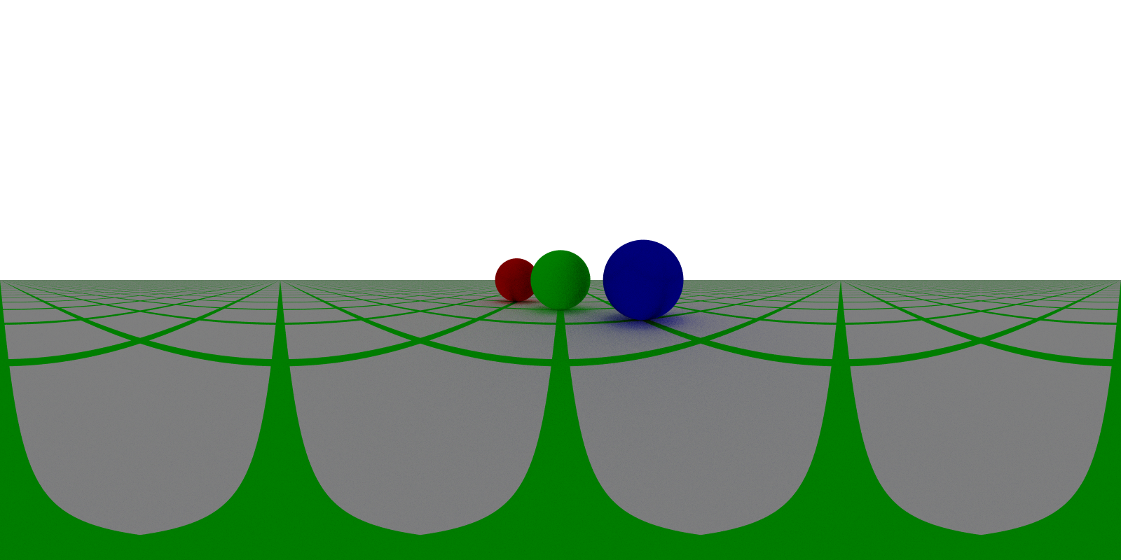 Figure 3: A view of the scene using the environment camera. Notice how the grid lines get distorted. In particular, since the camera is centered over an intersection point on the grid, we can see 4 lines going radially out to the horizon with the line traveling to the horizon behind the camera being bisected at the left/right edges of the image. Also notice that all the objects in the image are in focus, much like a pinhole camera.
Thin Lens Camera
As the name suggests, a thin lens camera makes use of the thin lens approximation which models the lens system as a single lens with spherical profiles where the thickness of the lens is small compared to the radius of curvature for the profiles. It is also the first of the camera models that utilize a finite aperture.
The basic process for generating rays using this model can be seen in fig. 4. First, we trace a ray originating from a given pixel and pass it through the center of the aperture to determine where it hit the focal plane. The distance to the focal plane and the size of the aperture can be set by the user. Once we know where a ray passing through the center of the aperture would intersect the focal plane, we sample a point on the aperture and shoot it towards the point on the focal plane. Consequently, all objects within the focal plane are in focus and objects outside of the focal plane will be increasingly out of focus the farther they are from the focal plane. See fig. 6 for examples of various focal lengths.
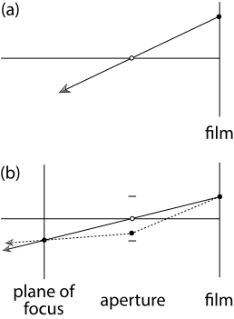 Figure 4 (PBRT figure 6.12): A diagram showcasing the basic approach used for the implementation of the thin lens approximation. (a) The pinhole camera model sends all rays through a single point. (b) For the thin lens approximation, we determine a point on the plane of focus by passing it through the center of the aperture just like we would for a pinhole. Then, we sample a point on the aperture and send it towards the point on the focal plane.
The blurriness of objects outside the plane of focus is determined by the size of the circle of confusion – points not on the focal plane will be imaged to a disk on the film plane. Objects will appear sharply in focus if the circle of confusion is smaller than the size of individual pixels. The circle of confusion is generally determined by the size of the aperture and the distance the film plane is from the focus of the lens. The circle of confusion for a particular object is also determined by the distance to the object from the lens. Notably, the change in the size of the circle of confusion is more dramatic for objects closer to the lens than the focal plane than for objects farther away (see fig. 5). The size of the circle confusion determines the depth of field of the image. A lens with a large aperture will have a higher depth of field than one with a smaller lens. For examples of this effect and the impact of aperture size, see fig. 7.
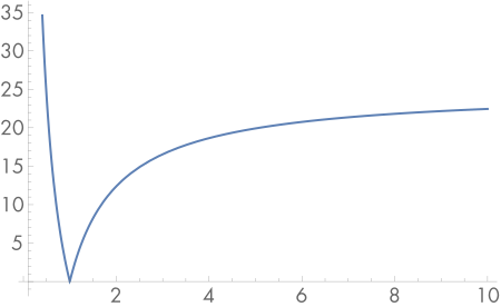 Figure 5 (PBRT figure 6.11): A graph of the size of the circle of confusion for a lens focused at 1 meter. The change in the size of the circle of confusion is more dramatic closer to the sensor than the distance to the focal plane and less so for points past it.
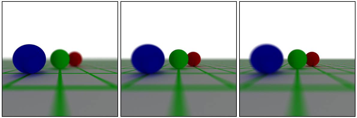 Figure 6: Various focal lengths for a thin lens camera with the aperture size set to 0.1. (Left) focal length set to 2. (Middle) focal length set to 3. (Right) focal length set to 4.
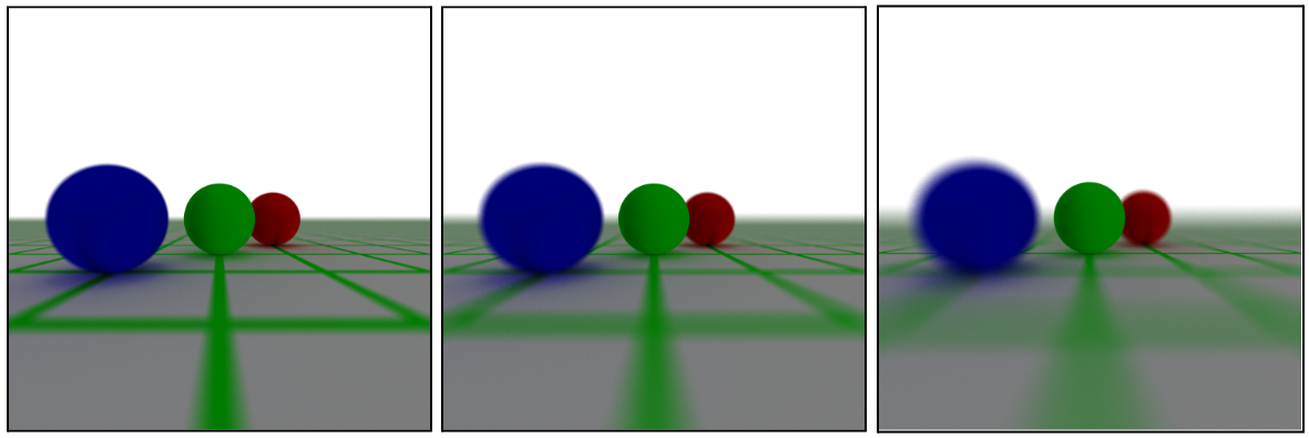 Figure 7: Various aperture sizes for a thin lens camera with the focal length set to 3. (Left) aperture size set to 0.05, (Middle) aperture size set to 0.1, (Right) aperture size set to 0.2.
Realistic Camera
A key advantage of ray tracing over traditional rasterization methods is the ability to accurately model the transportation of light through a scene. This can be extended to include accurate transport of light through a series of lenses as well. Consequently, it is possible to ray trace actual camera lenses and incorporate several realistic effects such as depth of field, aberration, distortion, and vignetting. Tracing real camera lenses is conceptually simple: if we assume our lens profiles are spherical, then we just need to trace a list of spheres and refract the ray at each intersection accordingly. And, it turns out that this is almost exactly how the lens elements are simulated.
The lenses are treated as a series of spherical interfaces and stored in a table (or more precisely, a vector of LensElementInterfaces) and the lenses are treated as extending to the left of the film plane along the negative z-axis. Each entry in the table lists the radius of the spherical element, the thickness of the element (i.e. the distance along the z-axis from the previous element), the index of refraction of the medium to the right of the interface, and the diameter of the aperture. The radius of the element can be positive or negative and is what determines if this element is concave or convex, i.e. if we should return the closer or further intersection point. Aperture stops (which block exiting rays) are represented as elements with 0 radius. The aperture diameter determines the radial extent from the z-axis that rays are allowed to intersect the element at before they are considered blocked. The aperture diameter of the first element is used to sample the possible directions that rays can be initialized in. The thickness of the first element is used to adjust the focus of the lens system.
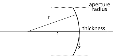 Figure 8 (PBRT figure 6.17): A diagram showing how lens interfaces are defined. The thickness is the distance along the negative z-axis from the previous interface to this one. The aperture radius determines the radial bounds of the lenses. If a ray intersects the element beyond those bounds, it fails to exit the lens system. The radius r is used to determine the curvature of the interface. In this case, r is a negative value so we intersect with the closer side of the sphere. The sphere is centered at the z-value of the interface plus the radius.
There are a number of performance enhancements we can utilize to ray trace the lenses compared to ray tracing normal objects in our scene. For one, we know the order of objects we are ray tracing so we do not need to perform intersection tests with multiple objects or bounding boxes. Instead, we just iterate through the lenses to trace them. Also, we can utilize specialized ray-sphere intersection code for the case where all spheres lie along the z-axis. This primarily saves us from having to do matrix transformations to move the elements into place. One other advantage of treating all lenses as lying along the z-axis is that we can trace the rays through the lenses in the lens coordinate system then do a single matrix transformation from the camera coordinates to the world coordinates.
For these renders, ray samples are given 10 attempts to exit the lens system before they are treated as having failed to exit the lens system and painted black. I.e., for each starting position on the sensor, we sample the first element’s aperture radius to determine the initial ray direction up to 10 times before giving up. The probability that a ray will exit the lens system is determined by the size of the exit pupil which dictates the range of positions at which a ray originating from a point on the sensor can exit the lens system from. Consequently, lens systems that have smaller exit pupils are more likely to end up dark as the current setup of the renderer treats any rays that fail to exit the lens system as black. One method to improve the efficiency of sampling exiting rays is to compute the exit pupil radially from the center of the lens. However, that has not been implemented for this report.
The following figures showcase a variety of lens systems. One common feature among each of these images is that they have been cropped to just the right size such that the image produced by the lenses fits within the bounds of the sensor. To produce these images, I manually adjusted the distance to the first lens element to set the focus and then adjusted the size of the sensor to encapsulate the whole image.
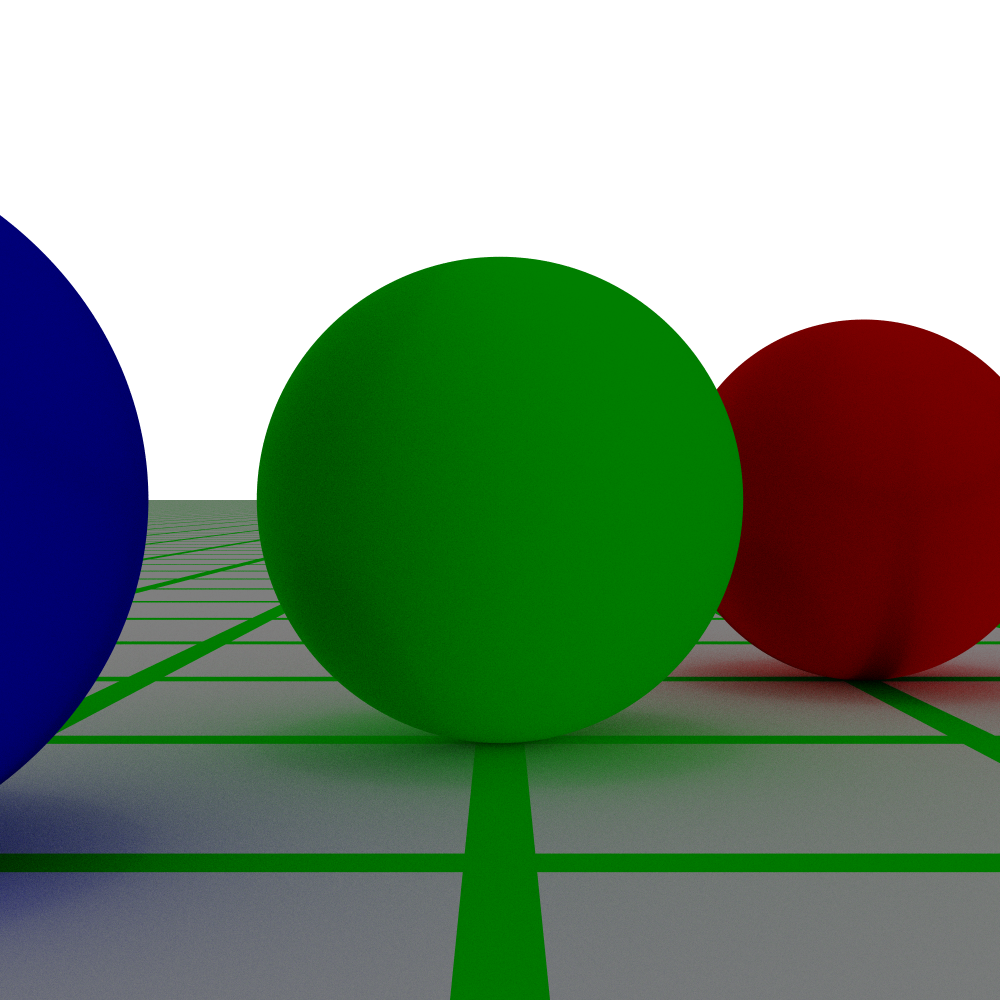 Figure 9: The no lens case for the realistic camera is set to approximate a pinhole camera. This was primarily used for testing. A physically accurate depiction would allow rays to travel in any direction over the whole hemisphere of directions away from the film plane.
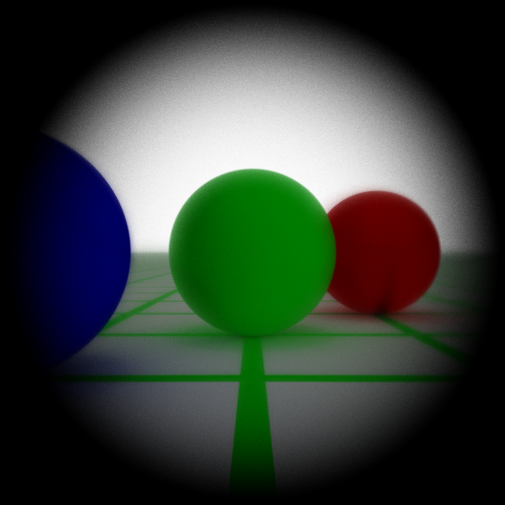 Figure 10: A true spherical lens made of two lens elements of the same radius and the aperture diameter set to match their radii.
 Figure 11: The same spherical lens but not placed far out of focus. In order to reduce the noise in this image, it was rendered with 512 samples per pixel instead of 256 like the other images.
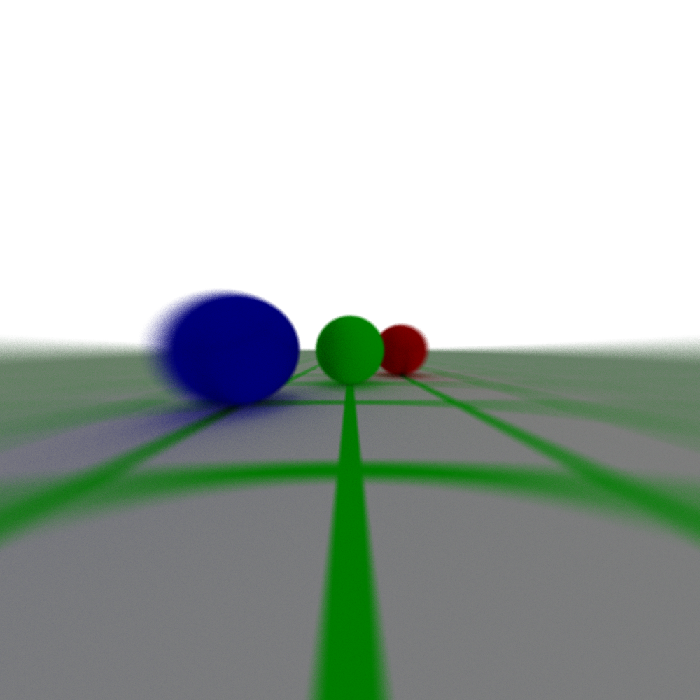 Figure 12: A single biconvex lens without any aperture stop. For reference the size of the aperture diameter is approximately 1/10th the radius of the lens elements. For this particular lens, the sphere at the center was in focus regardless of how far the lens was from the sensor but the field of view increased as the distance decreased (as we would expect as the cone of sampled directions per pixel gets larger).
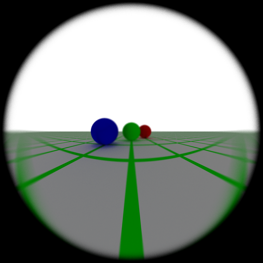 Figure 13: The same biconvex lens but with an aperture stop in the middle of the lens elements. This seems to dramatically change the behavior of the lens despite the fact that the distance from the first to the second lens element is still the same. One interesting thing to note about this and the prior lens is they do a good job showcasing aberration.
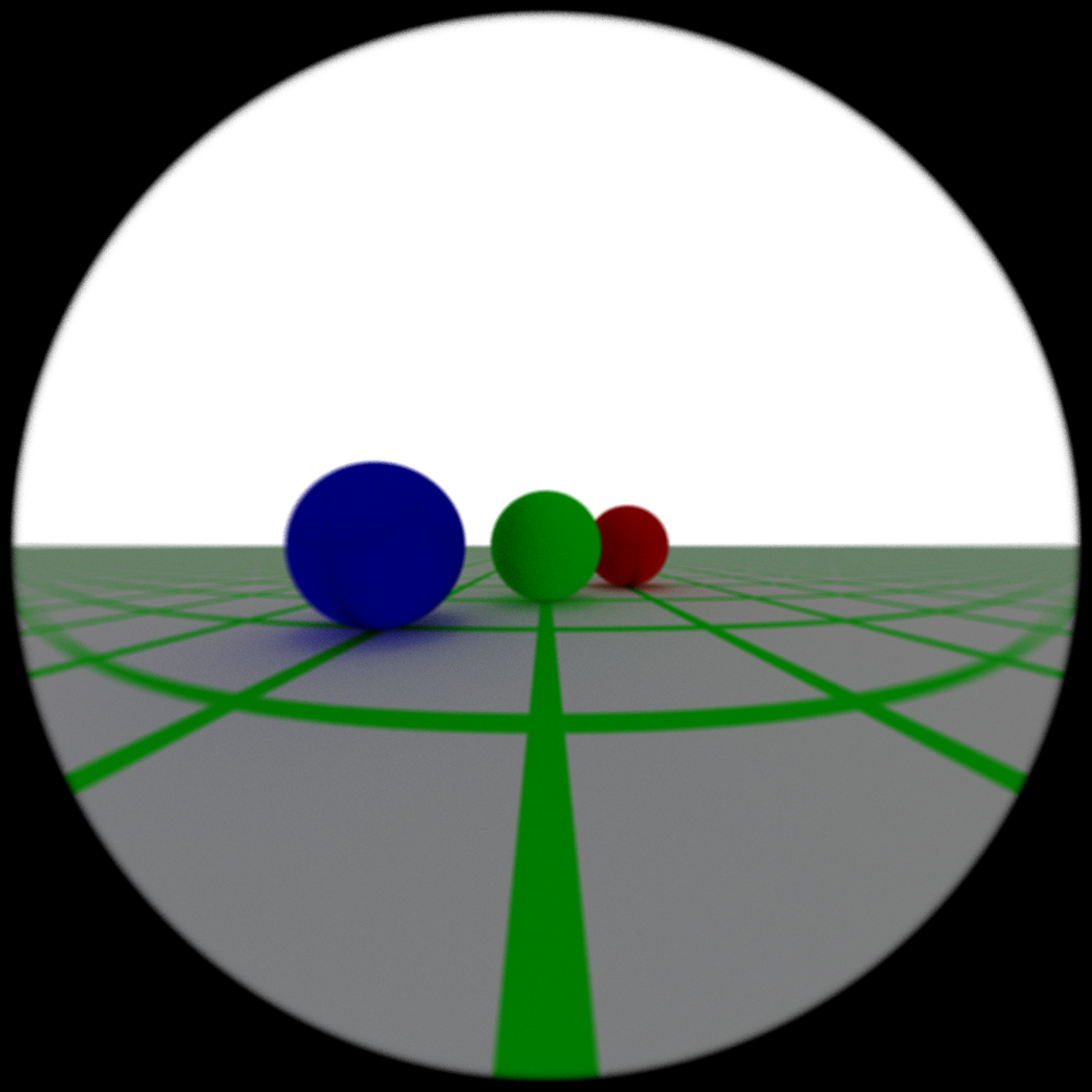 Figure 14: A biconcave lens with a very small aperture (1 mm!). If the aperture is any larger, everything becomes completely out of focus.
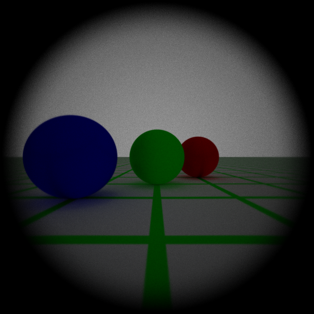 Figure 15: A wide angle lens taken from PBRT. It is very dim because many of the rays did not manage to exit the lens system, likely because this lens system has very small exit pupils.
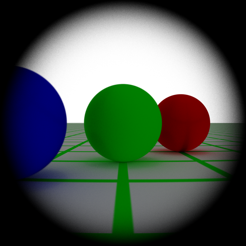 Figure 16: A Gaussian lens characterized which seems to keep all objects in focus and features quite strong vignetting. (Also looks quite a bit like the spherical lens in fig. 10).
 Figure 17: A fisheye lens. Features minimal aberration despite a very large field of view.
Future Directions
The camera models presented in this report are still just scratching the surface of the range of possible cameras and effects that can be simulated. For instance, the lens elements in this report were treated as purely spherical which meant that we could not have, for instance, non-spherical aperture stops or be able to simulate split diopter lenses like the ones discussed in the introduction. Also, total internal reflection for rays are completely ignored which are important for simulating effects such as lens flares. The current implementation also assumes that all wavelengths of light have the same indices of refraction which means effects such as chromatic aberration cannot be simulated properly.
There are also improvements that can be made to improve the efficiency of tracing the lenses. I have already mentioned that the exit pupil is not being calculated. Another improvement that is not currently working is an auto-adjustment of the focus using the thick lens approximation.