Panoramic Image Stitching

Image stitching is the process of combining several images of a scene taken from approximately the same viewpoint but at different angles to create a larger resulting image. One of the underlying assumptions of this process is that the fields of view of the images to be stitched slightly overlap. This assumption allows for the detection of common features within the images. The relative positions of the features allows for the calculation of a matrix transformation which describes how to warp one image to fit the coordinate system of another. Once the coordinate transformation is determined, the images can be warped, combined, blended together, and then cropped to produce a larger, panoramic image of the scene.

I decided to implement this process mostly from scratch as my final project for my Intro to Computer Vision course. So, let’s take a look at some of these steps in more detail. The following is a some-what shortened version of the final report I wrote for the project:

Determining Matching Points

The first step in image stitching is to get pairs of matching points between two images. What we ultimately want are pairs of coordinates from the two images that represent the same ‘features’ in both images. There are several options that exist but the most prominent and relevant method for this application is the Scale Invariant Feature Transform (SIFT), as described by David Lowe. The SIFT algorithm provides us with a set of unique keypoints in the image along with descriptors that uniquely identify each of the said keypoints. The keypoints and descriptors provided by the SIFT algorithm are scale, rotation, translation, and lighting invariant, making SIFT an excellent choice for matching. The general procedure for SIFT is to create a scale space of difference of gaussian (DoG) images and then search for local extrema in the scale space. The fact that it searches for extrema at various scales and levels of blur is what makes this procedure scale invariant. Once it finds the local extrema, it does some thresholding and pruning to remove less prevelant local extrema and removes local extrema along edges which are poorly localized (i.e., it is difficult to tell where along an edge a given feature might be). The next step of the SIFT algorithm is to create the descriptors. To do so, it first finds the prominent orientation of the region surrounding the position of the feature and ‘re-orients’ (so to speak) the surrounding region according to that prominent orientation. This process is what helps these features be rotationally invariant. Next, the descriptor itself is made by concatenating a series of histograms that represent the binned directions of 4x4 regions surrounding the feature position. In total, it looks 16 4x4 regions surrounding the feature position, each with 8 bins for direction, resulting in a unique 128 element descriptor for that keypoint. Then, to find matching features, we can compare the descriptors using a distance measure like the L2 norm (i.e., euclidean distance) and find the best sets of matching descriptors.

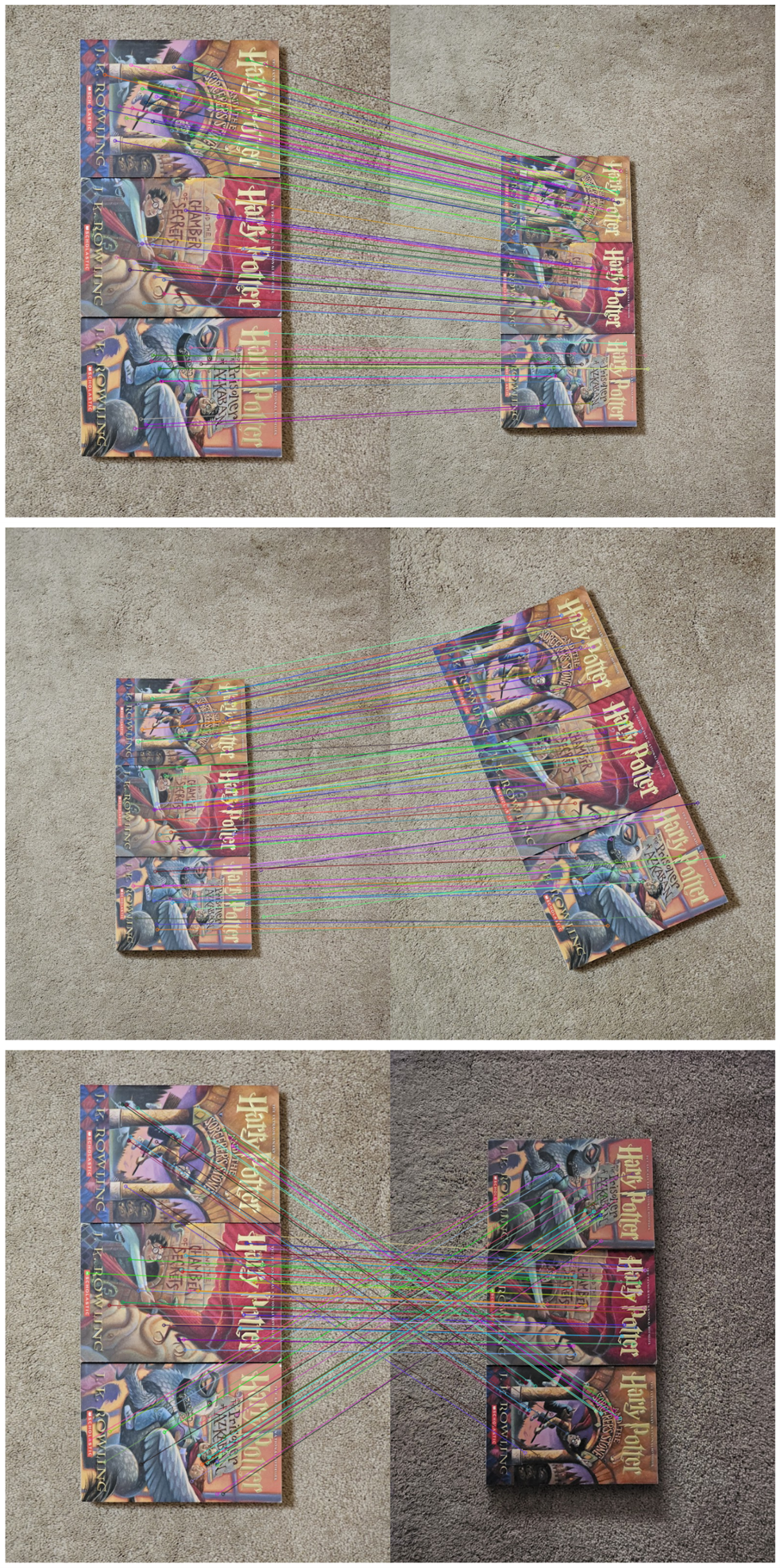
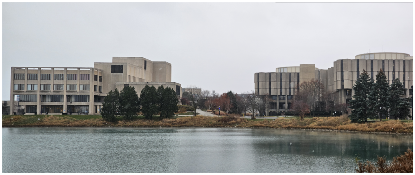
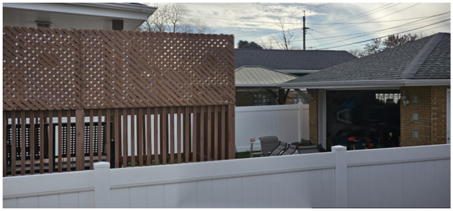
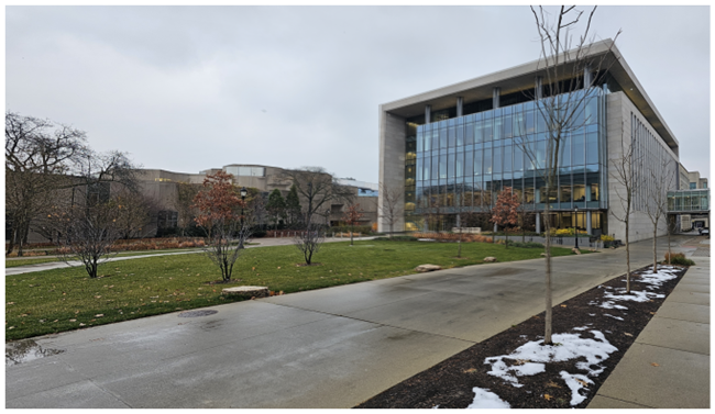
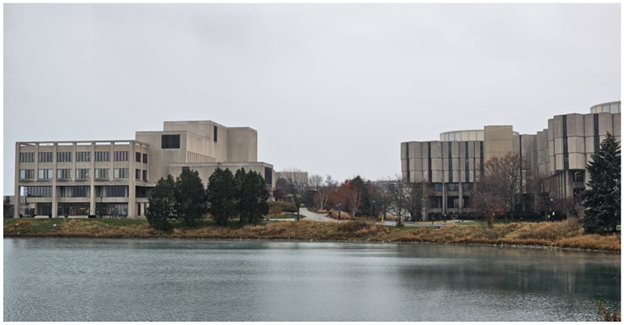
While I did try to implement the SIFT algorithm myself, none of my attempts were particularly successful (or even close, for that matter). Instead, since this algorithm was not the focus of the project, I decided instead to use the built-in OpenCV methods to determine SIFT keypoints and descriptors as well as OpenCV’s brute force matcher to find matching points. Figure 1 shows the SIFT algorithm in action, displaying the most prominent matches between the images at various scales, orientations, and lighting conditions.

Determining the Homography Matrix

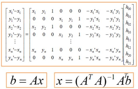
Once we have our pairs of matching points, we need to determine the matrix transformation that allows us to warp one image to match the perspective of the other image. This matrix transformation is also known as a homography matrix. My first attempt at solving this problem was to use psuedo inverse to do least squares using the setup that was shown in our class (see figure 2). However, I was not able to get this to work properly. At first, I thought the issue was that SIFT was returning noisy points so I moved on to implementing the next substep in the process: eliminating noisy matches using the Random Sample Consensus (RANSAC) algorithm.

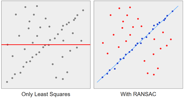
The RANSAC algorithm is a modification to least squares that allows us to extract prominent patterns in noisy data. See figure 3 for an example of its application on a 2D dataset. The general steps for the algorithm are as follows:

1. Randomly choose s samples.
   • Often, we choose s to be the minimum number of samples needed to fit our model. In this case, s = 4 since each pair of matching points gives us 2 coordinates and we only need 8 total values instead of 9 since we can normalize our homography matrix by the last element.
2. Fit your model to the chosen samples.
   • I.e., use least squares to compute the homography matrix for the chosen samples.
3. Apply the model to all points in the starting image to determine where the current model predicts the points will be when converted to the coordinate frame of the second image. Then, compare the predicted positions to the actual positions of the corresponding points in the second image and determine the number of inliers for the current model that are within some threshold. The particular threshold we choose is a hyperparameter.
4. Repeat steps 1-3 for n iterations.
   • n is a hyperparameter which we can adjust to be just enough for our maximum number of inliers to converge. This technically can be scaled by the number of matches since you can converge faster when you have fewer matches but for this project, hard coding it to 1000 seemed to work well enough for most cases, and 2000 worked for almost every case.
5. Choose the model with the highest number of inliers.
   • One thing to note is that, for my implementation, I stored the inliers every time I found a model with a new highest number of inliers. You could technically avoid storing it and simply store the indices of the matching points and then recompute the inliers, but this seemed more straightforward.
6. Optionally, fit the model to all the inliers.
   • I.e., once we have found a model that describes the most prominent pattern, we can note that the model is still only as accurate as our threshold. So, we can re-fit the model using the inliers to get a better fit to the detected pattern.

Going back to the earlier issue I was having, even after implementing RANSAC, I was still not getting a good homography matrix and was getting terrible results like those shown in figure 4. So, I decided to move on and used the built in OpenCV method ‘cv2.findHomography’ (which also uses RANSAC) to determine the homography matrix. It was not until after I got the later parts of the code working that I went back to try to fix my least squares fitting code. In the end, after some searching online, I came across homogeneous linear least squares and a formulation for determining the homography matrix from this paper by David Kriegman which suggested an alternate formulation for the A matrix and the use of singular value decomposition instead of traiditonal least squares. When I implemented that approach, I was getting much better matches.

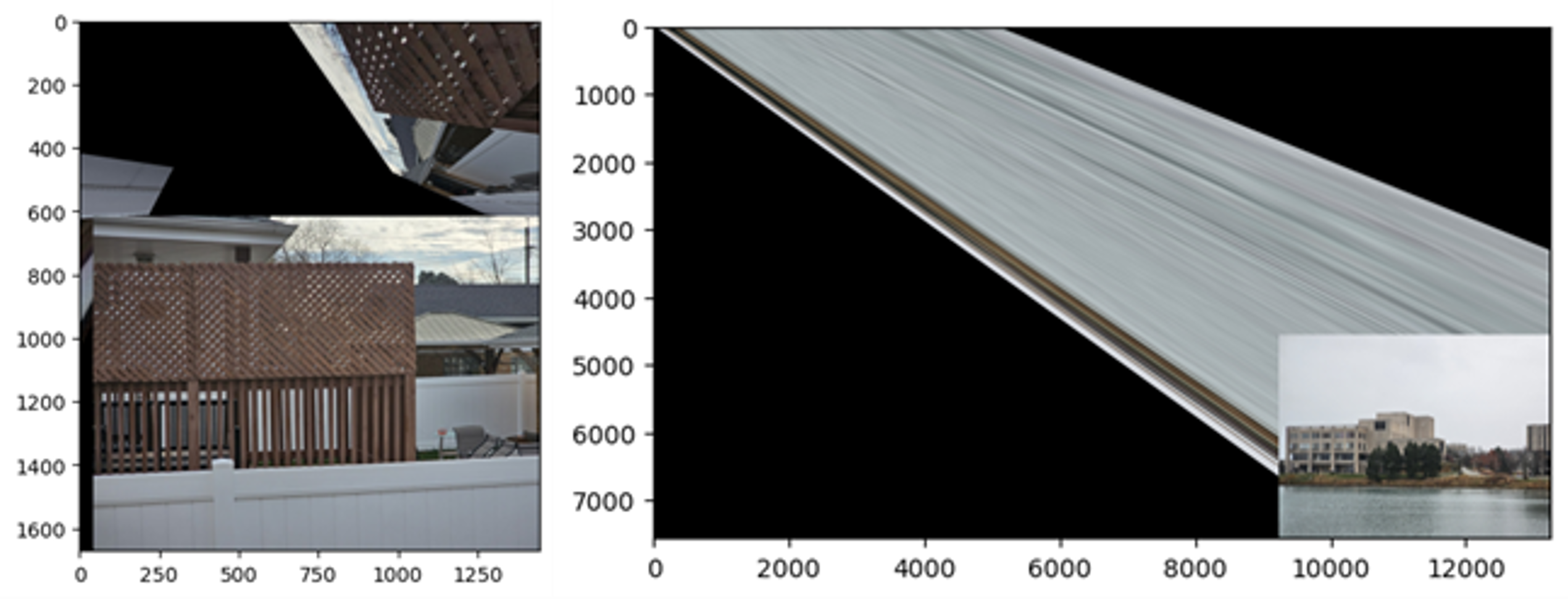
Image Stitching

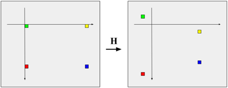
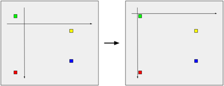
Determining New Bounds

The next step after determining the homography matrix is to actually combine the images together. To do so, the first step is to determine what the new bounds of the stitched image will need to be to encapsulate both the base image and the image that we will warp to overlay on top of the base image. To do so, we first apply the homography matrix to each of the 4 corners of the image we will warp. Then, using both the bounds of the warped image and the base image, we can determine a new set of bounds which encompasses both images. One implementation detail to make note of in this process is that the warped image bounds can be negative, so when we warp an image, we will also need to apply a transformation to the base image to move it with respect to the new basis.

Inverse Homography and Bilinear Interpolation

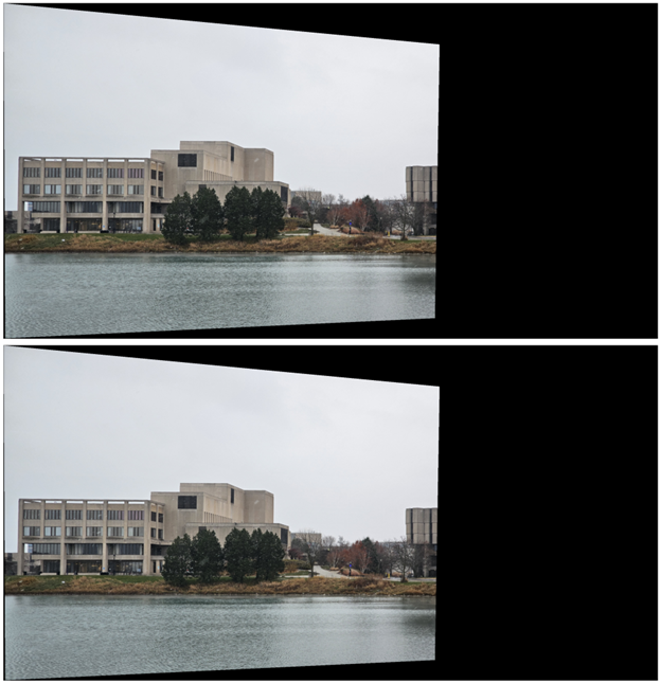
Once we know the new image bounds, we can start filling in the new image with the image we will warp. However, if we directly apply the homography to the initial image, not all points in the initial image will map to points in the warped version of the image. This issue is similar to the issue of resizing an image where we need to fill in the holes that would be produced if we simply scale up an image. To get around this, we instead apply the inverse homography to points in the warped image (or, more precisely, points within the new image bounds). If applying the inverse homography to a point in the new image bounds maps to a valid point within the bounds of the original image we are warping, then, we can do bilinear interpolation to determine the color of the pixel. Bilinear interpolation allows us to determine the color of the pixel by weighting according to the four closest pixels. In particular, we interpolate along x for the closest two pixels above the current position and the closest two pixels below it, then interpolate along y between those two x-interpolated values. Technically, this process is not required, especially since we have already taken care of the issue of having holes. However, for images where the warping is more severe, it should help remove jagged edges along lines in the image. However, in my testing, none of the warping for my test images was bad enough to produce any noticeable difference between the images which used interpolation and those which did not (see figure 6). Despite this, I opt to keep bilinear interpolation on by default since it appears to have minimal impact on performance. Instead, my implementation of warping is slow because I iterate through each pixel in the combined image using a for loop instead of parallelizing the process using something like numpy. I tried to do a more efficient implementation using numpy but was unsuccessful in all of my attempts so far.

Blending

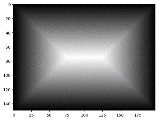
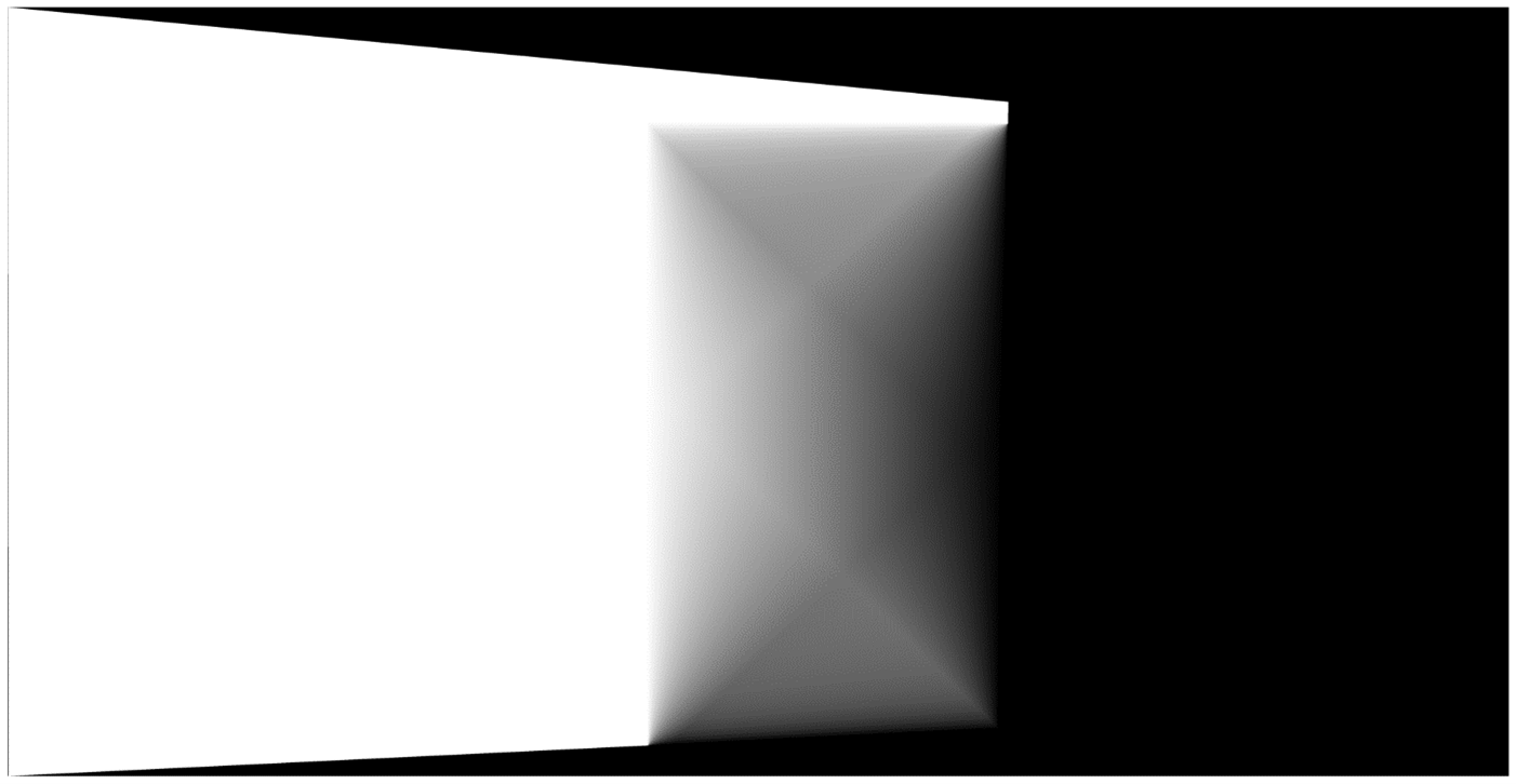
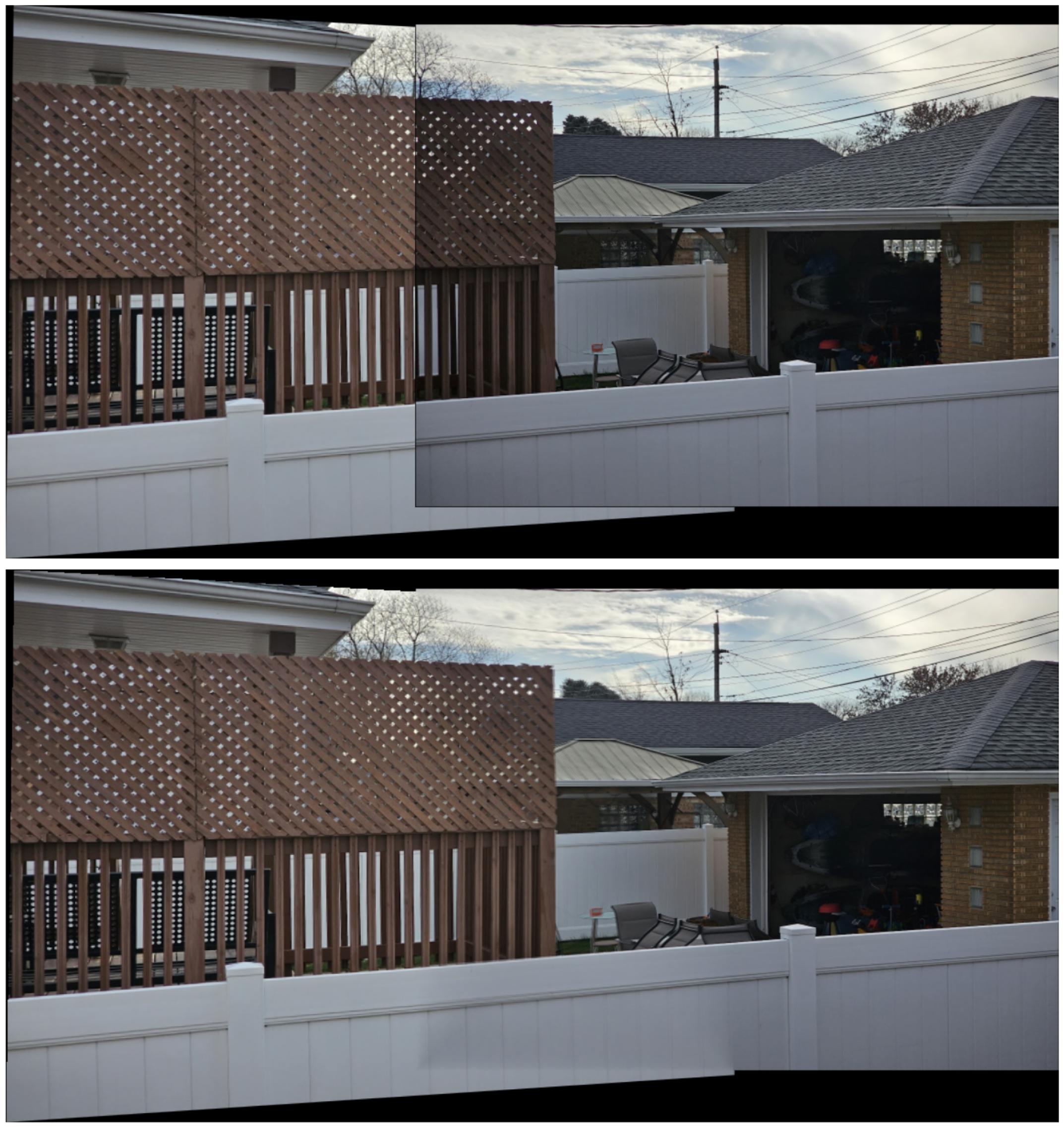
Once we have warped our image to match the coordinates of our base image, we can add in the base image to the stitch after transforming it into position for the new bounds. However, if we do this, we get a result like figure 7 where we can see a clearly defined border between where the two images overlap. This boundary is caused by slight lighting differences between the two images. These changes in lighting can be due to different exposures, vignetting, or even by something as simple as a cloud temporarily blocking some sun light. To address this, we can blend the images by applying weights to each image and then effectively interpolating between the images depending on the weight. In particular, we can create a weight matrix like seen in figure 8 for each of our images. We then apply the same transformation to our weights as we do to our original images. After that, we can create a sort of mask (as seen in figure 9) which determines how much of the original image to use in coloring a certain pixel versus how much of the new image should be used. Then, we color the image using that mask and the end result is a blended image with significantly less visible seams. See figure 10 for an example where this process works particularly well and figure 11 for another example where this process does not seem to work as well.

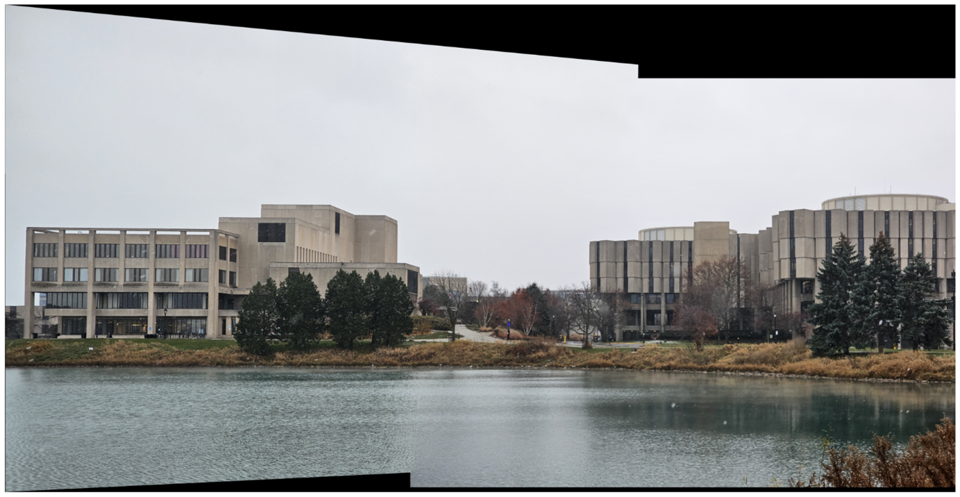
Cropping

The last step in the process of combining images is to crop the resulting image to remove invalid regions and produce a continuous rectangular region that encompasses the largest possible valid region. I first tried to implement clipping by working my way from the outside in, essentially stepping in along each direction until we find a region that is fully valid. However, I found that for situations like figure 11, there is no point along the y direction where all rows of the image are valid due to the odd shape of the warped image bounds (i.e., the top left and bottom left bounds of the warped image are at different x-values). So instead, I tried the opposite approach, I grow a rectangular region out from the center of the image. In particular, within a while loop, I check if growing the starting region by some value to the right produces a region that is entirely valid (i.e. has all non-zero values). If it is valid, I move on to the next side, i.e., the bottom. However, if it is not valid, I divide the rate to check along the right by 2 before moving on to the next side. I repeat this process for all 4 sides over 1 iteration. By repeating this process, I can quickly grow the region at what is effectively an O(n log(n)) rate and find the maximum size valid region. However, there are a few caveats to this function. For one, I chose to grow to the right first because I espect that direction to be valid all the way to the right. If, instead, we grow along the bottom first, we can end up in situations where we get stuck on ‘ledges’ of valid regions like those in figure 10. One hack to get around this is to set a starting size which hopefully surpasses those ledges though I found that growing along the right first is more consistent and does not require setting a starting size.

Multiple Images

For my implementation, I added the ability to stitch 3 images as well. One goal when I set out on this project was to be able to stitch an arbitrary number of images. You can see this goal reflected in the fact that I created an Image class that stores the homography matrix of the image. After the fact, the design to use the Image class turned out to be useful for storing SIFT features as well but I was unable to create an effective way to combine an arbitrary number of images. This is because when combining arbitrary numbers of images, we need to determine which images to stitch and in which order to stitch them. In practice, this should involve storing the homography matrices of each image such that when we warp a new image to another image which has already been warped, we can combine their homography matrices. However, determining the order to match images proved a difficult task and so I hard coded the process for stitching two images and stitching three images by assuming that the center image provided for a three image stitch is the intended base image (and also the central image).

Results

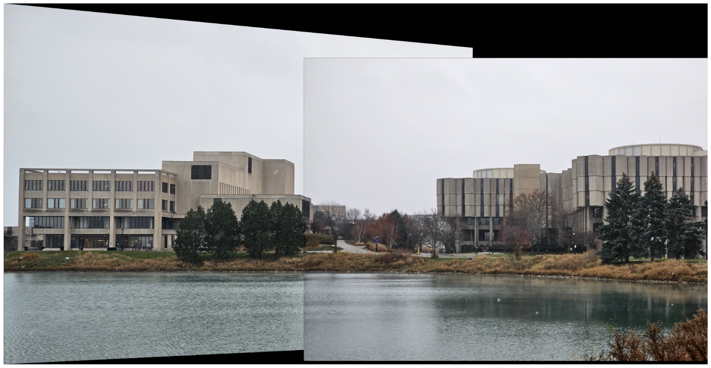
Two Image Stitches (fig. 12)

Three Image Stitches (fig. 13)

Analysis

My implementation of this allows for the user to easily switch between using OpenCV methods and entirely using my own implementation. Both seem to produce indistinguishable results which suggests that the end results of my functions for computing homography and warping images are doing near-identical operations as the ‘official’ functions. However, one area that my functions are lacking in are speed. For reference, to process the top image in figure 13 using OpenCV methods took 26 seconds in total for both RANSAC and image warping. However, my implementation took 519 seconds!

Another thing I noticed was that the initial image size has a very large impact on processing time. In particular, anything above about 2k pixels along each axis leads to prohibitively long processing times for my implementation and painfully long using OpenCV. Even OpenCVs SIFT implementation tends to ramp up, going from an almost instant 0.1 seconds to several minutes. This makes sense since we are using a Brute Force matcher, and if we have several thousand matches for a large image as opposed to a few hundred, then we have exponentially more pairs of matches to compare. Also, RANSAC takes longer since we need to apply the homography matrix to all matching pairs and compute the distances between their predicted and true positions to determine if they are inliers. Image warping also scales exponentially with image size since we have to apply the transformation to each pixel.

One major issue that may be visible in the final images that I have not mentioned yet is that for several of the images, the objects seem to be doubled up in the overlapped region or at least be blurrier in the overlapped region. This is because the homography transforms are likely not providing a good enough match and the images are therefore not perfectly overlapping. I found this issue to be more prevelant in lower resolution images which we should expect since they effectively have a lower sampling rate (i.e., coarser bins) for determining positions. For cases like the bottom image of figure 12, it also seems that the camera itself may not be perfectly calibrated, potentially introducing some non-linear transformations that are not accounted for with our linear homography transformations.

Future Work

The first order of business to improve this implementation would be to add proper mutli-image support rather than hard coding the process for particularly stitching 2 or 3 images. This would involve determining which images should be matched with which other images and managing all the compounding homography matrices. Additionally, figuring out a way to account for non-linear transformations may prove beneficial in reducing the inaccuracies in the homography transforms. As a side note, I did attempt to increase the number of iterations for RANSAC but the number of matches capped out and refused to improve. We should expect this since there will only be a certain number of maximum inliers for a given threshold. However, it may be possible to get better results by fine tuning the threshold or adjusting the number of samples s per iteration. Other areas of improvement may be to implement more advanced blending techniques to help reduce seams or maybe even pre-process images to equalize their brightnesses. Finally, it may be worthwhile to investigate how to make my implementations of finding matches and warping more efficient so that I can approach the speed of the native OpenCV implementations.